How Is Gauge R&R Calculated? A Worked Example

The short answer

Gauge R&R is calculated by splitting the spread in repeated measurements into repeatability (one person, one gauge, measured again) and reproducibility (different people, same parts). Add the squares of the two and take the root to get GRR. Then compare GRR with the total variation or with the tolerance. In the example below GRR is 24.7 per cent of total variation, which is a marginal result, not a pass.

The method below follows the average and range approach that the AIAG Measurement Systems Analysis manual (fourth edition) describes. We checked the AIAG [MSA manual page](https://www.aiag.org/training-and-resources/manuals/details/MSA-4) on 1 November 2026: the fourth edition is current and the page names no newer one. We paraphrase the method and copy none of the manual's tables or forms. The arithmetic in this worked example was run in Node and every input is printed here, so you can repeat it.

What a gauge R&R study measures

Every measurement has two parts: the real size of the part and the error of the measuring system. A gauge R&R study estimates the error part. It does not tell you whether the gauge is "accurate" in the sense of matching a master. That is bias, which has its own study.

Two kinds of error make up GRR:

• Repeatability (equipment variation, EV): the spread when one appraiser measures the same part several times with the same gauge.
• Reproducibility (appraiser variation, AV): the extra spread between appraisers, such as one person pressing harder on a micrometer.

The usual design uses 10 parts that cover the whole process spread, 3 appraisers and 2 or 3 trials each, measured in random order and blind to the part number. Our example uses 10 parts, 3 appraisers and 2 trials, which gives 60 readings. The part is a turned shaft with a drawing size of 12.000 mm plus or minus 0.050 mm, so the tolerance is 0.100 mm. The gauge is a digital micrometer that reads to 0.001 mm.

The data

The readings are in millimetres:

Step 1: repeatability (EV)

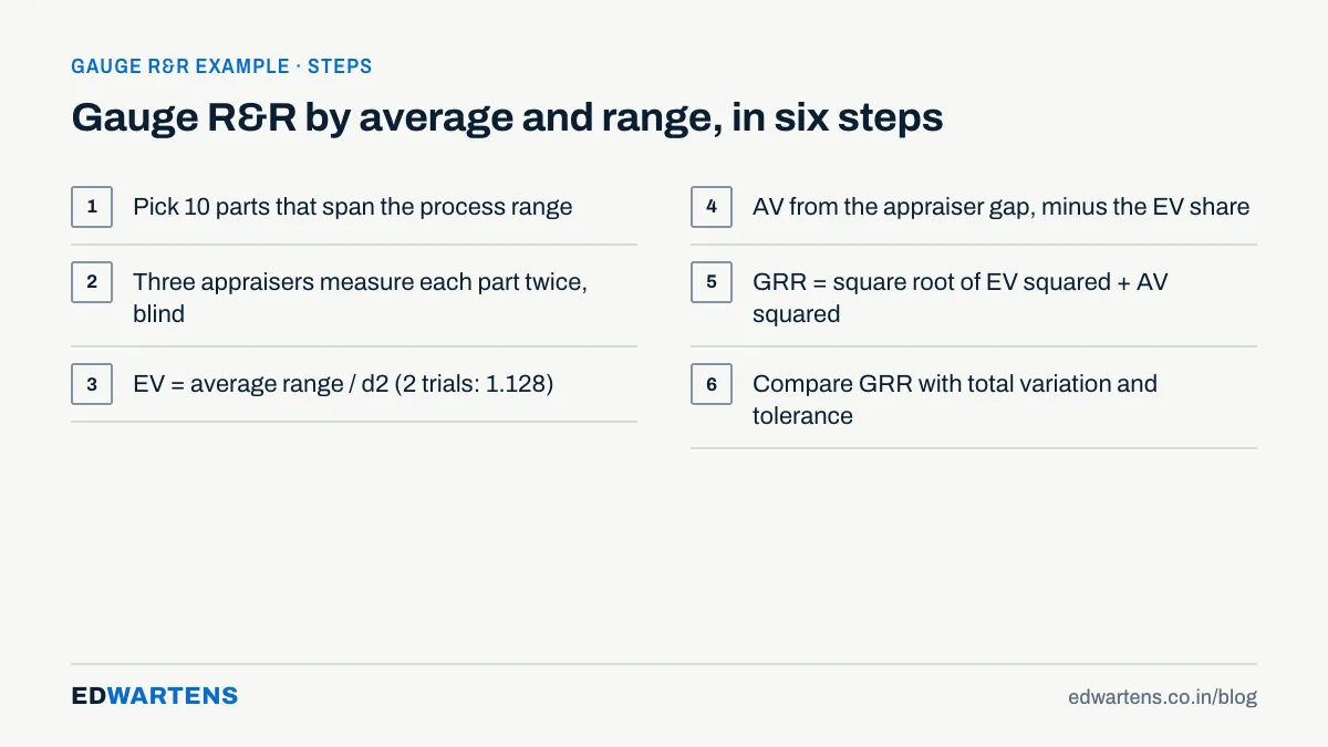
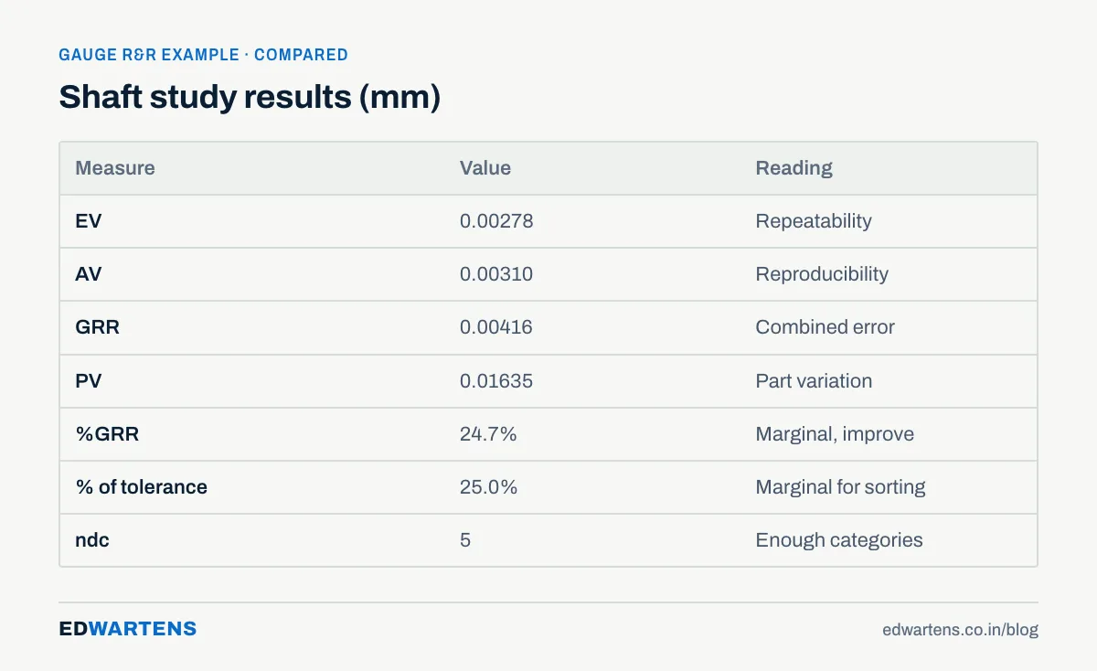
For each appraiser, find the range of the two trials on every part, then average those ten ranges. Appraiser A averages 0.00390 mm, B 0.00280 mm and C 0.00270 mm. The grand average range is (0.00390 + 0.00280 + 0.00270) / 3 = 0.003133 mm.

Divide by the constant d2 for the number of trials. For 2 trials d2 is 1.128, so EV = 0.003133 / 1.128 = 0.00278 mm. The AIAG manual tabulates slightly different constants, so a hand answer can differ from its tables in the last digit.

Step 2: reproducibility (AV)

Average all 20 readings each appraiser took: A is 11.99985 mm, B is 12.00330 mm and C is 11.99795 mm. The gap between the highest and lowest is 12.00330 - 11.99795 = 0.00535 mm. For three appraisers d2 is 1.693.

1. (0.00535 / 1.693)^2 = 9.986e-6
2. EV^2 / (parts x trials) = 0.00278^2 / 20 = 3.86e-7
3. AV = square root of (9.986e-6 - 3.86e-7) = square root of 9.600e-6 = 0.00310 mm

The subtraction removes the share of the appraiser gap that repeatability alone would cause. If the number under the root were negative, you would set AV to zero.

Step 3: GRR, part variation and total variation

GRR is the root of the sum of squares: the square root of (0.00278^2 + 0.00310^2) = 0.00416 mm.

For part variation, average all six readings of each part. The smallest part average is part 1 at 11.97483 mm and the largest is part 9 at 12.02517 mm, so the range is 0.05033 mm. For ten parts d2 is 3.078, so PV = 0.05033 / 3.078 = 0.01635 mm.

Total variation is the root of GRR squared plus PV squared: 0.01687 mm.

Step 4: judge the result

Three numbers decide whether the gauge is good enough.

The AIAG guidance, as it is usually summarised, reads like this. Customers can set their own limits, so read your customer's requirement first.

Our shaft study sits in the middle band. The gauge could stay in use for a feature that is not critical, with a plan to improve it. For a safety characteristic you would not accept 24.7 per cent.

The split tells you where to act. Appraiser variation (18.4 per cent of total variation) is a little larger than equipment variation (16.5 per cent). Appraiser B reads about 0.005 mm higher than appraiser C on average. So the first fix is a written method: where on the shaft to measure, how much to tighten the thimble and how to clean the anvil. Appraiser A also has the widest ranges, 0.00390 mm against 0.0028 and 0.0027, so A needs a short coaching session before the study is repeated.

The ANOVA method on the same data

The average and range method is quick but ignores whether appraisers and parts interact. The ANOVA method treats parts, appraisers and their interaction as sources of variance. Run on these 60 readings, the interaction is not significant. F is 0.79 and p is 0.693, well above the 0.25 cut-off that AIAG-style practice uses. So it is pooled into the error term. The ANOVA result is a GRR standard deviation of 0.00384 mm, 25.0 per cent of total variation, 23.1 per cent of tolerance and ndc 5. The two methods agree closely, which is what you expect from a clean data set. JASP and R can run the ANOVA for free, and a spreadsheet can do it with a little patience.

Mistakes that make a study meaningless

• Parts that do not span the process. If all ten parts are nearly the same size, part variation is tiny and %GRR looks terrible. Pick parts across the whole range, including some near each limit.
• Appraisers who know the part number. They remember the first answer. Randomise the order and hide the numbers.
• A gauge that cannot resolve the tolerance. A resolution coarser than about a tenth of the tolerance cannot pass. Our micrometer reads 0.001 mm against a 0.100 mm tolerance, which is 1 per cent.
• Measuring on different days or warm parts. Temperature and wear add variation that the study then blames on people.
• Ignoring a negative AV. It means appraiser differences are smaller than repeatability would suggest, so set it to zero and say so.

Why quality teams in India need this

Automotive suppliers in Pune, Chennai and the Gurugram belt often have to show measurement system studies inside a production part approval package. A quality engineer who can run and explain a study in a customer meeting saves a resubmission. Our AIAG-VDA FMEA guide for automation engineers shows the risk tools that sit beside this study. Our Six Sigma for manufacturing engineers post says where statistics-driven methods help and where they waste time. For the chart side of the same toolbox, the NIST e-Handbook explains control charts and its gauge R&R section covers measurement studies. JASP is a free statistics program for the ANOVA version.

Practise it free

The free SPC and MSA: Control Charts, Capability and Gauge R&R course teaches gauge R&R by the average and range method and by ANOVA. It has 10-part, 3-appraiser worked problems and attribute agreement. It also covers resolution, bias, linearity and stability, so you can judge a gauge before you study it. Everything can be repeated in Excel or LibreOffice Calc.

It is a free course with a verifiable certificate of completion, and anyone can check a certificate on our verification page. It is not a CPD or professional credential, it does not replace the AIAG manual your customer names, and EDWartens is not affiliated with AIAG. Start the SPC and MSA course when you are ready.

If you would rather practise this on PLC training panels with an instructor, see our PLC course in Bangalore for the syllabus and duration.

Frequently asked questions

Q: How is gauge R&R calculated?
A: Measure 10 parts with 3 appraisers and 2 or 3 trials each. Equipment variation comes from the average range of the trials divided by d2, appraiser variation from the gap between appraiser averages, and GRR is the root of their squares. Divide GRR by total variation or by the tolerance to get a percentage.

Q: What is an acceptable gauge R&R?
A: Under 10 per cent of total variation is generally acceptable. From 10 to 30 per cent it may be acceptable, depending on the use and the cost of a better gauge. Over 30 per cent is not acceptable. Your customer may set a stricter limit, so check it.

Q: What is the difference between repeatability and reproducibility?
A: Repeatability is the variation when one person measures the same part repeatedly with one gauge. Reproducibility is the extra variation between different people measuring the same parts. Together they make gauge R&R.

Q: How many parts, appraisers and trials do I need?
A: The common design is 10 parts, 3 appraisers and 2 or 3 trials. The parts must cover the real process spread, and the order must be random and blind.

Q: Should I use percent of total variation or percent of tolerance?
A: Use percent of total variation to judge whether the gauge can support process control. Use percent of tolerance to judge whether it can sort good parts from bad. Report both, and say which multiplier you used.

Q: Can I do a gauge R&R study in Excel?
A: Yes. The average and range method needs only averages, ranges and four constants. JASP or R can run the ANOVA method for free.